• 
• • 
  • 
  • 
  • 

Thank you for visiting our webpage. Here, we briefly introduce scanning nonlinear dielectric microscopy, a novel and unique microscopy that we have been developing for almost these two decades. This microscopy, shortly named ‘SNDM’, was originally targeted to ferroelectric materials and has a unique feature that is capable of imaging polarization distribution of sample surfaces in nanometer resolution. SNDM has already been in practical use and commercially available. We are now working for getting higher resolution and presented new applications of this microscopy as described in the following pages. In the first page, we briefly introduce the principle of SNDM, which is a common basis of various types of SNDM.

It is well known that matter is classified into conductors, semiconductors, and insulators by its electrical conductivity. The insulators, also called dielectrics, do not conduct electric current under the influence of an electric field. On the other hand, the dielectrics can be polarized by the electric field. In a macroscopic sense, the same amount of positive and negative surface charges is induced on one surface side and the opposite side perpendicular to the field, respectively. Microscopically, electrically charged particles, such as atomic nuclei, electron, and ions, constituting the materials cannot be freely moved but displaced from their equilibrium position due to Coulombic force. This phenomenon is called dielectric polarization. The amount of displacement is macroscopically characterized so-called dielectric constants and they are different in different materials.

Let us consider a simple model of polarization consisting of one positive charge and negative one connecting by a spring. Here, we assume the material has polarization without an external field, or spontaneous polarization, such as ferroelectric and pyroelectric materials. Inside this material, the positive charges are displaced toward the field and negative charges shift in the opposite direction. If the field is weak, the displacement would be proportional to the intensity of the field. In this case, dielectric constant can be considered as a proportional constant connecting the displacement and intensity of field．However, if the field has larger intensity, the situation can be different. Actually, literalistic treatment of a dielectric constant as ‘constant’ is a kind of the 1st order or linear approximation of a nonlinear electric response. In reality, the dielectric constants are not constants and varied depending on the external field．To be more precise, a nonlinear response of electric displacement D can be described by the Taylor expansion for an electric field E as follows.

We call the coefficients of nonlinear terms, such as ε₃, ε₄, …, nonlinear dielectric constants．ε₂ is here linear dielectric constant, or dielectric constant in an usual sense．SNDM can measure these nonlinear constants.

What would be evaluated through the measurement of nonlinear dielectric constants? Actually, the signs of odd-numbered constants ε₃, ε₅，… are changed depending on the direction of the polarization（please recall a D-E hysteresis loop of ferroelectric material, if you know）．This means that the direction of spontaneous polarization in a ferroelectric material can be determined through the measurement of nonlinear dielectric constants.

One way to measure nonlinear dielectric constants of a dielectric material is to make a capacitor using the material and then measure its capacitance variation to an applied field. For simplicity, let us consider a parallel plate capacitor. If we apply an external field E=E_pcos ω_pt between the two electrodes, the capacitance variation from the original capacitance is described by the equation in the figure above. This implies that capacitance is varied in a nonlinear and periodic manner with the same period as the sinusoidal field. According to this relation, a signal proportional to ε₃, the lowest order nonlinear dielectric constant, can be acquired through the measurement of the fundamental frequency component of the capacitance variation. In the same way, a signal proportional to ε₄ can be acquired from the second harmonic component. However, you might be still suspicious that the capacitance variation is too small to detect. Actually, nonlinear dielectric constant is so much smaller than the linear dielectric constant. The capacitance variation caused by nonlinear dielectric constants is typically less than 1/1000000 of the original capacitance.

The key to detect small capacitance variation is to transform capacitance variation to frequency shift of a LC oscillator and utilize frequency modulation (FM) and demodulation. The LC oscillator can be made by connecting an external inductor to the parallel plate capacitor and a feedback amplifier for exciting self-oscillation. Then, we have a LC oscillator oscillating at its eigenfrequency f0, which is described as follows:

Here C and L denote using capacitance and inductance of the inductor. This equation implies that, if the capacitance is slightly varied due to nonlinear dielectric constants, then the eigenfrequency shift is caused. In general, frequency measurement is useful, because it can be precisely measured using simple and moderate equipment. In addition, since frequency shift can be extracted using frequency mixing technique, we can use very high frequency LC oscillator for improving the sensitivity to capacitance variation （This is the same as why audio signal around 1kHz can be extracted from satellite broadcasting using 10GHz）．

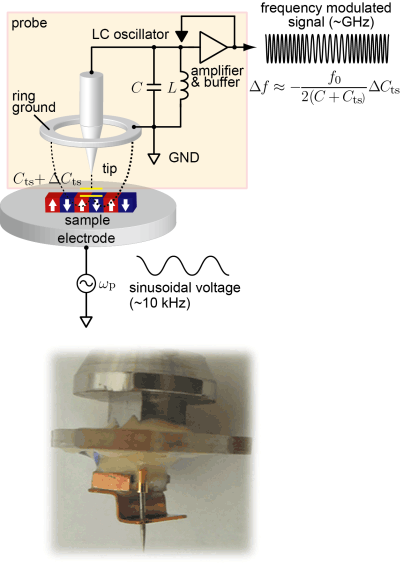
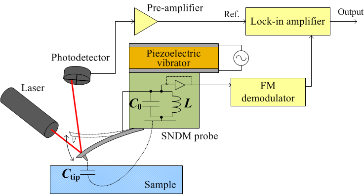
Instead of metal electrodes, you can use a metal tip for the measurement of a two dimensional map of polarization on a sample surface. That is, one of the two electrodes in the parallel plate capacitor is replaced by a metal tip shown in the next picture. By scanning over the surface and plotting ε₃ on each lateral position, polarization distribution can be acquired. Therefore, SNDM can be classified as a member of scanning probe microscopy．The probe of SNDM consists of a grounded ring electrode, sharp metal tip, external inductance and capacitance, and feedback amplifier. The capacitance is composed along the electric field originating from the metal tip, going through the sample, and returning to the ring ground. The LC oscillator then consists of tip-sample capacitance, and external inductor and capacitor. The probes developed by our group are extremely sensitive to capacitance variation of up to 10^-23 Farad.

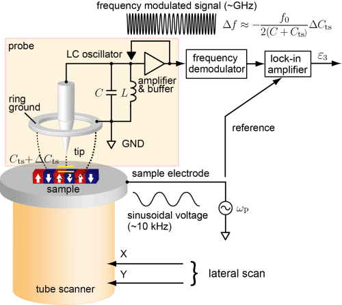
A schematic diagram of SNDM is shown in the next figure. The frequency of a sinusoidal field is typically the order of 10 kHz and it is applied between a sample stage and a ring electrode grounded together with a metal tip. The frequency shift is demodulated by a FM detector and a nonlinear dielectric constant is acquired by a lock-in amplification of a corresponding frequency component. The direction of polarization beneath the tip is determined by the polarity of the acquired ε₃ signal relative to the applied field. Thus, by scanning over the sample surface and mapping ε₃ on the corresponding position, two dimensional distribution of polarization can be obtained.

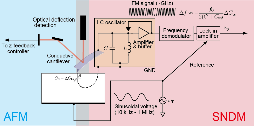
Like SNDM, a family of microscopic techniques using a scanning probe that detects any local (physical, chemical, electrical, ...) state of a sample for obtaining an image is called scanning probe microscopy (SPM). As mentioned above, SNDM can also be classified as a member of the SPM family. SNDM can be combined with other SPM methods, allowing the microscopic evaluation of samples from multiple aspects. As a typical example, the combination of atomic force microscope (AFM) and SNDM is shown below. AFM uses a microcantilever with a sharp tip at the free end as a probe, and the force acting between the tip of the probe and the sample surface is detected locally. When the sample surface is scanned, the force changes according to the surface topography. Then, a topographic image can be obtained by the feedback-control of the sample height to keep the detected force constant. By using a conductive-coated cantilever, we can perform SNDM imaging simultaneously. Through the simultaneous acquisition of a topographic image and a spontaneous polarization distribution image, it becomes possible to discuss the relationship between the surface structure and spontaneous polarization. In addition, AFM is useful for keeping a constant experimental condition in SNDM imaging. The contact force can be well regulated during scanning, which also prevents damage to the sample and probe. Thus, the combined use of AFM and SNDM is very effective.

AFM has several operation modes. Contact mode AFM has been mainly used with SNDM and has already been applied to various samples in the different fields of research. However, in contact mode AFM, since the probe is always in contact with a sample, a large lateral force acts on the probe and the sample. This causes problems such as damaging soft samples and dragging samples weakly adsorbed on substrates. In addition, especially when using an ultra-shape tip for high resolution, the tip is likely to be damaged. In such cases, it is effective to combine SNDM with intermittent contact AFM, where the tip contacts with the sample surface only intermittently. Since it becomes easier to maintain the sharpness of the tip, intermittent contact SNDM can also be expected to contribute to higher resolution. Intermittent contact AFM dramatically reduces the lateral forces, greatly reducing probe and sample damage. Note that the capacitance variation detected by SNDM attenuates rapidly when the tip is slightly separated from a sample surface. We need longer contact time or an appropriate signal detection scheme not to reduce signal-to-noise ratio in the SNDM channel.

Can SNDM observe linear permittivity distribution in addition to nonlinrear permittivity distribution? The answer is “yes.” Our SNDM can also observe linear permittivity distribution with a minor modification in the setup.

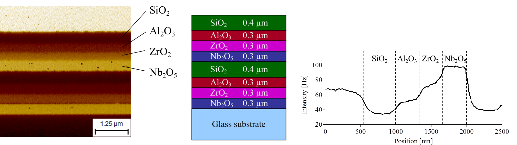
As mentioned earlier, the conventional SNDM (∂C/∂V-SNDM) detects capacitance variation induced with ac bias application to the sample. In contrast, ∂C/∂z-SNDM detects the capacitance variation induced by mechanical vibration of the cantilever. The observed capacitance variation corresponds to the sample permittivity in the ∂C/∂z mode because the tip-sample capacitance is sensitive to the sample permittivity when the probe tip is in contact with the sample surface, and is insensitive to the sample permittivity when the probe tip is retracted sufficiently from the sample surface. Therefore we can obtain a linear permittivity image by monitoring the SNDM output signal with keeping the vibration amplitude of the cantilever constant. The following figure shows an example of a permittivity image for multilayer oxide films observed with this method.

Static domain structures are observed in the conventional study on ferroelectrics using SNDM. However, we are often interested in the dynamics of polarization switching as well as the static domain structures. SNDM is also useful for studying the dynamics of such polarization switching.

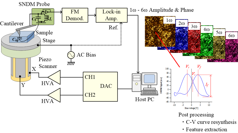
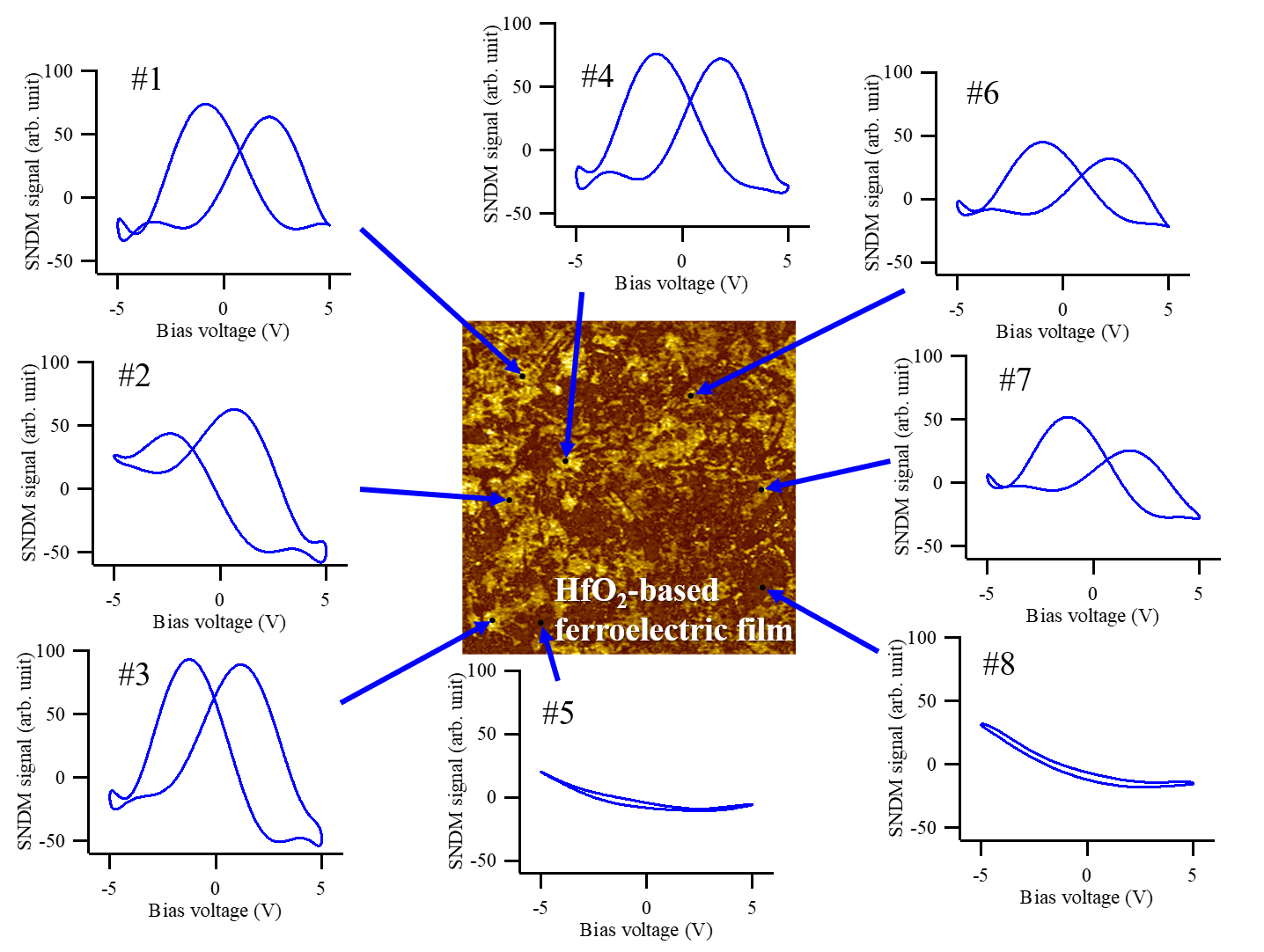
When observing static domain structures, a small AC bias below the polarization switching voltage is applied to the sample, whereas, when examining the dynamics of polarization switching, an AC bias with a relatively large amplitude exceeding the polarization switching voltage is applied. Then, a response waveform corresponding to a large capacitance variation due to polarization switching is observed at the output of the FM demodulator in the SNDM setup. At this time, if the applied AC bias is plotted on the horizontal axis and the SNDM response signal on the vertical axis (C-V plot), a butterfly-like curve characteristic of ferroelectrics is drawn. By analyzing this butterfly curve in detail, various information on the nanoscale polarization switching of ferroelectrics can be obtained.

In summary, we have reviewed the principle of SNDM. In the following pages, we show various applications of this microscopy such as super high density ferroelectric probe data storage, evaluation of miniaturized semiconductor devices, and noncontact atomic scale dipole moment imaging of various surfaces and interfaces.

A book has been published that explains in detail from the principle of SNDM to its application.

Paperback ISBN: 9780128172469
eBook ISBN: 9780081028032
https://www.elsevier.com/books/scanning-nonlinear-dielectric-microscopy/cho/978-0-12-817246-9（Elsevier）
https://www.amazon.co.jp/Scanning-Nonlinear-Dielectric-Microscopy-Investigation/dp/0128172460（amazon）